Tukey’s test plot in adas.utils

Abstract

The new version 1.1.1 of the adas.utils package includes a new function to plot the results of Tukey’s test.

Rationale

The new version v1.1.1 of the adas.utils package includes a new function to plot the results of Tukey’s test. The function is called ggTukey and it is used to plot the results of Tukey’s test provided by the stas::TukeyHSD function.

John W. Tukey

The standard stats::TukeyHSD function returns an S3 object that has the print and plot methods. The result of the plot method, though, is honestly not really appealing. Let’s see how it works, by loading a dataset and running a Tukey’s test on it. We load an online dataset by using the adas.utils::examples_url function¹, and we begin with a simple boxplot of the data.

library(tidyverse)
library(adas.utils)

data <- examples_url("anova.dat") %>% 
  read.table(header=TRUE) %>% 
  mutate(Cotton=factor(Cotton)) %>% 
  glimpse()

Rows: 25
Columns: 3
$ Cotton      <fct> 15, 15, 15, 15, 15, 20, 20, 20, 20, 20, 25, 25, 25, 25, 25…
$ Observation <int> 1, 2, 3, 4, 5, 1, 2, 3, 4, 5, 1, 2, 3, 4, 5, 1, 2, 3, 4, 5…
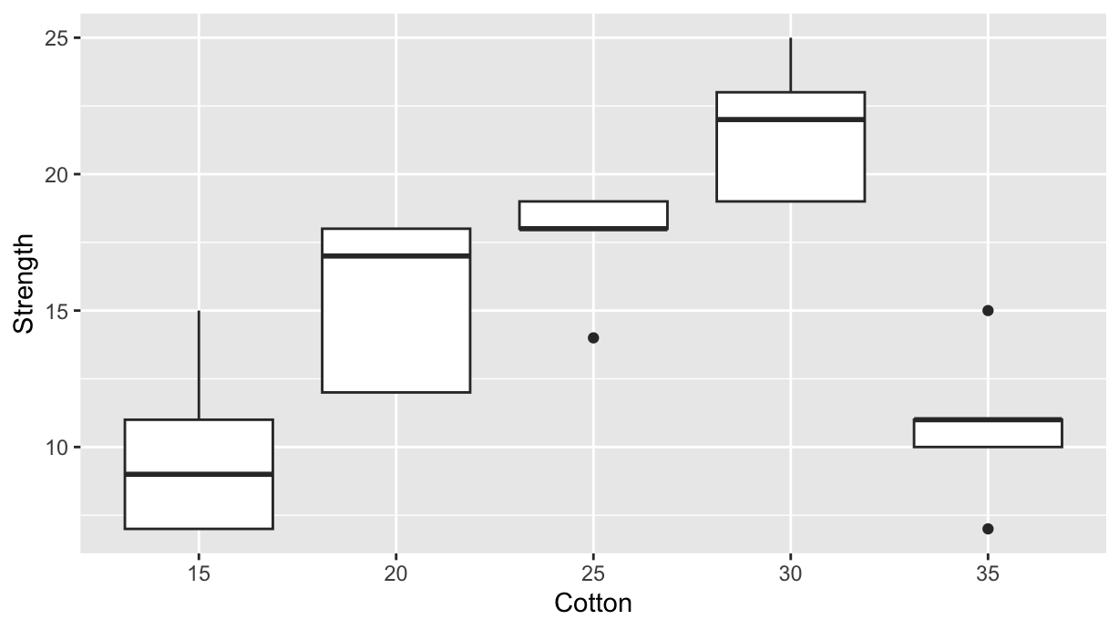
$ Strength    <int> 7, 7, 15, 11, 9, 12, 17, 12, 18, 18, 14, 18, 18, 19, 19, 1…

data %>% 
  ggplot(aes(x=Cotton, y=Strength, group=Cotton)) +
  geom_boxplot()

The Tukey’s test is built by using the aov function and the TukeyHSD function. The results are then plotted by the plot method of the TukeyHSD object:

data %>% 
  aov(Strength ~ Cotton, data=.) %>%
  TukeyHSD() %>% 
  plot()

The biggest problem with plot.TukeyHSD is that the labels of the differences are often partially hidden if there are many groups or the plot is too squat. This is the main reason for implementing an analogous function based on GGplot2 in adas.utils.

Enter ggTukey

Labels are much more readable in the ggTukey plot. Let’s see how it works:

data %>% 
  aov(Strength ~ Cotton, data=.) %>%
  TukeyHSD() %>% 
  ggTukey()

There’s actually more: you can also pass to ggTukey the data frame and the formula to be used in the aov model:

data %>% 
  ggTukey(Strength ~ Cotton)

Which is nicely more tidiverse-y and readable, isn’t it?

Now let’s look at a different, slightly more complex dataset:

data <- examples_url("battery.dat") %>% 
  read.table(header=TRUE) %>% 
  mutate(Material=factor(LETTERS[Material]), Temperature=factor(Temperature)) %>%
  glimpse()

Rows: 36
Columns: 6
$ RunOrder      <int> 34, 25, 16, 7, 8, 1, 26, 36, 6, 13, 3, 31, 27, 29, 12, 1…
$ StandardOrder <int> 1, 2, 3, 4, 5, 6, 7, 8, 9, 10, 11, 12, 13, 14, 15, 16, 1…
$ Temperature   <fct> 15, 70, 125, 15, 70, 125, 15, 70, 125, 15, 70, 125, 15, …
$ Material      <fct> A, A, A, B, B, B, C, C, C, A, A, A, B, B, B, C, C, C, A,…
$ Repeat        <int> 1, 1, 1, 1, 1, 1, 1, 1, 1, 2, 2, 2, 2, 2, 2, 2, 2, 2, 3,…
$ Response      <int> 130, 34, 20, 150, 136, 25, 138, 174, 96, 155, 40, 70, 18…

This one shows discharge test results for batteries with different dielectric materials (qualitative factors) and operating at different temperatures (quantitative factors). So inn this case we have two predictors. We want to create a set of Tukey’s tests for each level of Material. We need to pass ggTukey with the formula Response ~ Temperature (for the aov model) and the splt argument with another, one side formula that specifies the grouping factor: ~Material. In a terse and clear way, we can write:

data %>% 
  ggTukey(Response ~ Temperature, splt=~Material)

And that was not possible with the standard plot.TukeyHSD method, at least not in two lines of code.

That’s all, folks!

Footnotes

1. This function can load any data file listed on https://paolobosetti.quarto.pub/data